Showing posts with label data wrangling. Show all posts

Sunday, March 11, 2018

Are you smarter than a fifth grader?

"the editorial principle that nothing should be given both graphically and in tabular form has to become unacceptable" - John W. Tukey

Back to school

In the United States, most fifth grade students are learning about a fairly powerful type of visualization of data. In some states, it starts at an even younger age, in the 4th grade. As classwork and homework, they will produce many of these plots:


They are called stem-and-leaf displays, or stem-and-leaf plots. The left side of the vertical bar is the stem, and the right side, the leaves. The key or scale is important as it indicates the multiplier. The top row in the image above has a stem of 2 and leaves 0,6 and 7, representing 20, 26 and 27. Invented by John W. Tukey in the 1970's (see the statistics section of part II and the classics section of part V of my "ex-libris" series), few people use them once they leave school. Doing stem-and-leaf plots by hand is not the most entertaining thing to do. The original plot was also limited to handling small data sets. But there is a variation on the original display that gets around these limitations.

"Data! Data! Data!"

Powerful? Why did I say that in the first paragraph?

And why should stem-and-leaf plots be of interest to students, teachers, analysts, data scientists, auditors, statisticians, economists, managers and other people teaching, learning or working with data? There are a few reasons, with the two most important being:
  • they represent not only the overall distribution of data, but the individual data points themselves (or a close approximation)
  • They can be more useful than histograms as data size increases, particularly on long tailed distributions


An example with annual salaries

We will look at a data set of the salaries for government employees in Texas (over 690,000 values, from an August 2016 snapshot of the data from the Texas Tribune Salary Explorer). From this we create a histogram, one of the most popular plot for looking at distributions. As can be seen, we can't really tell any detail (left is Python Pandas hist, right is R hist):


It really doesn't matter the language or software package used, we get one very large bar with almost all the observations, and perhaps (as in R or seaborn), a second tiny bar next to it. A box plot (another plot popularized by John Tukey) would have been a bit more useful here adding some "outliers" dots. And, how about a stem-and-leaf plot? We are not going to sort and draw something by hand with close to 700,000 values...

Fortunately, I've built a package (python modules plus a command line tool) that handles stem-and-leaf plots at that scale (and much, much larger). It is available from http://stemgraphic.org and also from github (the code has been available as open source since 2016) and pypi (pip install stemgraphic).
So how does it look for the same data set?


Now we can see a lot of detail. Scale was automatically found to be optimal as 10000, with consecutive stems ranging from 0 to 35 (350000). We can read numbers directly, without having to refer to a color coded legend or other similar approach. At the bottom, we see a value of 0.00 (who works and is considered employed for $0 annual income? apparently, quite a few in this data set), and a maximum of $5,266,667.00 (hint, sports related), we see a median of about $42K and we see multiple classes of employees, ranging from non managerial, to middle management, upper management and beyond ($350,000+). We've limited the display here to 500 observations, and that is what the aggregate count on the leftmost column tells us. Notice also how we have a convenient sub-binning going on, allowing us to see which $1000 ranges are more common. All this from one simple display. And of course we can further trim, zoom, filter or limit what data or slice of data we want to inspect.

Knowing your data (particularly at scale) is a fundamental first step to turning it into insight. Here, we were able to know our data a lot better by simply using the function stem_graphic() instead of hist() (or use the included stem command line tool - compatible with Windows, Mac OS and Linux).

Tune in next episode...

Customers already using my software products for data governance, anomaly detection and data quality are already familiar with it. Many other companies, universities and individuals are using stemgraphic in one way or another. For everybody else, hopefully this has raised your interest, you'll master this visualization in no time, and you'll be able to answer the title question affirmatively...

Stemgraphic has another dozen types of visualizations, including some interactive and beyond numbers, adding support for categorical data and for text (as of version 0.5.x). In the following months I'll talk a bit more about a few of them.


Francois Dion
@f_dion

N.B. This article was originally published on LinkedIn at:

https://www.linkedin.com/pulse/you-smarter-than-fifth-grader-francois-dion/

Tuesday, February 27, 2018

Stemgraphic v.0.5.x: stem-and-leaf EDA and visualization for numbers, categoricals and text


 Stemgraphic open source


In 2016 at PyDataCarolinas, I open-sourced my stem-and-leaf toolkit for exploratory data analysis and visualization. Later, in October 2016 I had posted the link to the video.


Stemgraphic.alpha


With the 0.5.x releases, I've introduced the categorical and text support. In the next few weeks, I'll be introducing some of the features, particularly those found in the new stemgraphic.alpha module of the stemgraphic package, such as back-to-back plots and stem-and-leaf heatmaps:


But if you want to get started, check out stemgraphic.org, and the github repo (especially the notebooks).

Github Repo

https://github.com/fdion/stemgraphic


Francois Dion
@f_dion

Thursday, April 13, 2017

Readings in data and databases

Recent readings (can you guess/decipher some of them?)

I've been fairly quiet on this particular blog this year. Beside a lot of data science work, I've done presentations at meetups and conferences, including a recent tutorial on "Getting to know your data at scale" at the IEEE SouthEastCon 2017. Notebooks will be posted on github soon.

But, in the meantime...

Ex-libris

Something else I've been doing is publishing a few articles here and there. Just recently, I started a 6 part series on LinkedIn called "ex-libris" of a Data Scientist. I think many readers of this blog will appreciate this series, and particularly this first installment on "data and databases":

"ex-libris" of a Data Scientist - Part i

It covers a good variety of books on the subject, some pretty much must read for whatever corner of the computer science world you live in. Also of interest will be the Postgres, Hadoop and graph database pointers and a list of over 20 curated must read papers in the field.

Python specific books will show up in part IV.


Francois Dion
@f_dion

Thursday, October 20, 2016

Stemgraphic, a new visualization tool

PyData Carolinas 2016

At PyData Carolinas 2016 I presented the talk Stemgraphic: A Stem-and-Leaf Plot for the Age of Big Data.

Intro

The stem-and-leaf plot is one of the most powerful tools not found in a data scientist or statistician’s toolbox. If we go back in time thirty some years we find the exact opposite. What happened to the stem-and-leaf plot? Finding the answer led me to design and implement an improved graphical version of the stem-and-leaf plot, as a python package. As a companion to the talk, a printed research paper was provided to the audience (a PDF is now available through artchiv.es)

The talk


Thanks to the organizers of PyData Carolinas, videos of all the talks and tutorials have been posted on youtube. In just 30 minutes, this is a great way to learn more about stemgraphic and the history of the stem-and-leaf plot for EDA work. This updated version does include the animated intro sequence, but unfortunately the sound was recorded from the microphone, and not the mixer. You can see the intro sequence in higher audio and video quality on the main page of the website below.

Stemgraphic.org

I've created a web site for stemgraphic, as I'll be posting some tutorials and demo some of the more advanced features, particularly as to how stemgraphic can be used in a data science pipeline, as a data wrangling tool, as an intermediary to big data on HDFS, as a visual validation for building models and as a superior distribution plot, particularly when faced with non uniform distributions or distributions showing a high degree of skewness (long tails).

Github Repo

https://github.com/fdion/stemgraphic


Francois Dion
@f_dion


Sunday, November 29, 2015

Box office plot (the other kind)

Tables can obfuscate understanding

And we have a follow up question on the Pandas read_html wikipedia James Bond article. Namely, how do we quickly visualize the data.

It is true that the table we had in the previous article doesn't help us with easily seeing the trend (it wasn't the purpose). Even trimming this down to just the Bond movie title and box office normalized to 2005 million $ doesn't help us that much, even with the minimum and maximum highlighted:


TitleBox office.1
1Dr. No448.8
2From Russia with Love543.8
3Goldfinger820.4
4Thunderball848.1
5You Only Live Twice514.2
6On Her Majesty's Secret Service291.5
7Diamonds Are Forever442.5
8Live and Let Die460.3
9man with !The Man with the Golden Gun334.0
10spy who !The Spy Who Loved Me533.0
11Moonraker535.0
12For Your Eyes Only449.4
13Octopussy373.8
14view !A View to a Kill275.2
15living !The Living Daylights313.5
16Licence to Kill250.9
17GoldenEye518.5
18Tomorrow Never Dies463.2
19world !The World Is Not Enough439.5
20Die Another Day465.4
21Casino Royale581.5
22Quantum of Solace514.2
23Skyfall879.8


Same data, only better

The absolute minimum to get pandas to plot a graph in a Jupyter notebook (I'm assuming you have enabled inline graphics by using %matplotlib inline) is to use the dataframe method plot, ie. df.plot():


The result of df.plot() with no other options

It usually does the right thing, including a readable legend, and picking only the columns that have numbers or dates. We could also have done a bar graph, but in this case would not have been as readable.

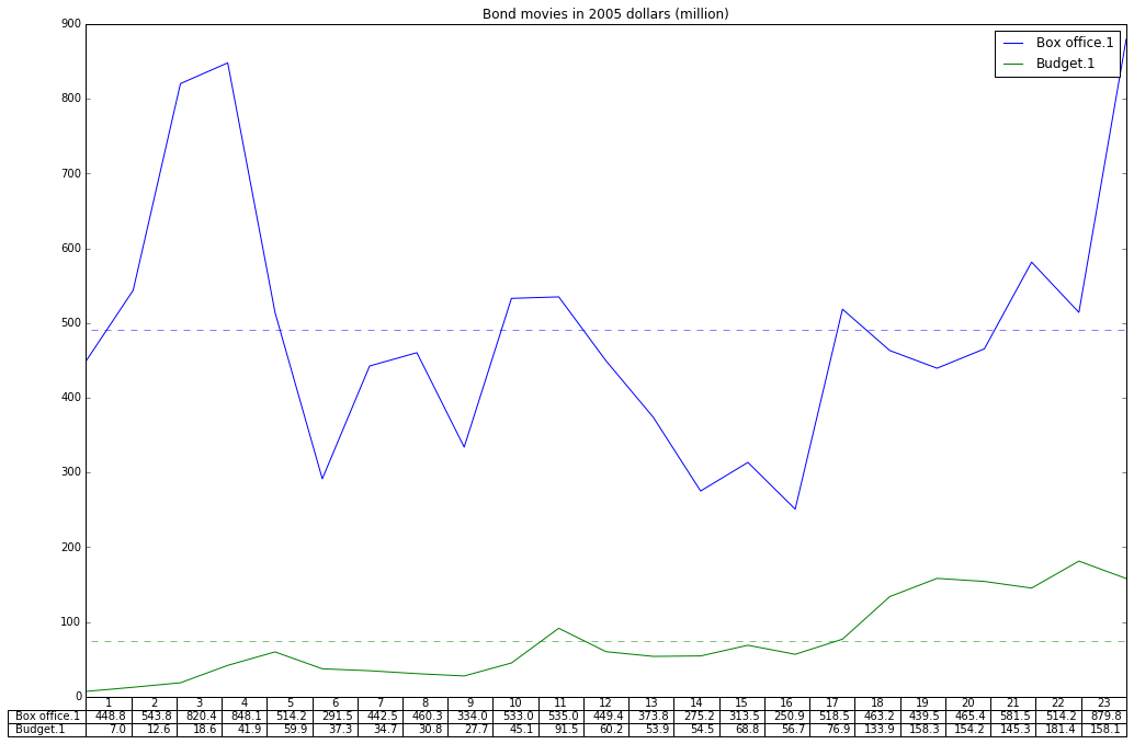
Now, let's add a few elements to this. For one thing, I'd like to not only plot a line graph (default) but to add a table directly under the graph. Since we'll have this table under the X axis, let's remove the tick values on X by using xticks=[].

I think we all can agree that a graph should have a title, so we will add that too. And finally, let's make it a bit larger.

ax = df.plot(table=True, xticks=[], title="Bond movies in 2005 dollars (million)", figsize=(17,11))

And how about adding the average value as a dotted horizontal line for the box office?

ax.hlines(y=df.mean()[0], xmin=0, xmax=23, color='b', alpha=0.5, linestyle='dashed', label='Box office average')

Might as well do it for the budget too. So in all we have:

ax = df.plot(table=True, xticks=[], title="Bond movies in 2005 dollars (million)", figsize=(17,11))
ax.hlines(y=df.mean()[0], xmin=0, xmax=23, color='b', alpha=0.5, linestyle='dashed', label='Box office average')
ax.hlines(y=df.mean()[1], xmin=0, xmax=23, color='g', alpha=0.5, linestyle='dashed', label='Budget average')

So, how does it look?
Final result - click to see full size image


The jupyter notebook can be found on github: pandas_bond.ipynb

Francois Dion
@f_dion

Wednesday, November 25, 2015

Bond. James "import pandas" Bond

It all started when...

    [friend] I'm trying to get this table on wikipedia from python...

[me] Sure. What module are you using?

    [friend] BeautifulSoup, but man, this is hard. It's this url...

[me] Wait, this is not a Coursera assignment you are asking me to do, is it?

    [friend] No, no. I saw this thing using a different programming language and I want to do it in Python.

[me] Ok, sounds reasonable.

The URL

The basic URL that documents James Bond movies on wikipedia is at: https://en.wikipedia.org/wiki/List_of_James_Bond_films but the URL he sent me was: https://en.wikipedia.org/w/index.php?title=List_of_James_Bond_films&oldid=688916363 and hence why it looked like a assignment.


Let me pause for a brief second on this subject. I'm a big fan of reproducible research, and selecting a specific revision of a document is an excellent idea. This page will never change, whereas any given normal URL on wikipedia changes all the time.

I'll have some of that BeautifulSoup

My friend mentioned he was trying to use BeautifulSoup but facing some challenges. BeautifulSoup and lxml are the usual suspects when it comes to doing web scraping (and using requests itself to pull the data in). But I have to admit, most of the time I don't use any of these. You see, I'm lazy, and typically these solutions require too much work. If you want to see what I'm talking about, you can check using-python-beautifulsoup-to-scrape-a-wikipedia-table

I don't like to type more code than I need to. At any rate, the goal was to get the web page, parse two tables and then load the data in a pandas data frame to do further analysis, plots etc.

Enter the Pandas

And it's not even the Kung Fu Panda, just good old Pandas, the data wrangling tool par excellence (https://pypi.python.org/pypi/pandas/0.17.1).

Everybody knows, I hope, that it has a superb support for loading excel and CSV files. It's why Python is the number 1 data wrangling programming language.

But what about loading tables from wikipedia web pages, surely there is nothing that can simplify this, is there? If you've attended all PYPTUG meetings, you already know the answer.

 import pandas as pd  
   
 wiki_df = pd.read_html("https://en.wikipedia.org/w/index.php?title=List_of_James_Bond_films&oldid=688916363", header=0)  

read_html returns a list of dataframes, with each table found on the web page being a dataframe. So to access the box office table on this page, we have to look at the second dataframe, the first being the warning table at the top of the page. Since it is 0 indexed we refer to it with wiki_df[1]. We don't want line 0 because that's sub headers, and we don't want the last two lines because one is a movie that's just been released and the numbers are not in yet, and the other one because it's a total column. How do we do this? Good old Python slices:

 df = wiki_df[1][1:24]  

And that's it, seriously. One line to ingest, one line to cleanup.

The result

Title Year Bond actor Director Box office Budget Salary of Bond actor Box office.1 Budget.1 Salary of Bond actor.1
1 Dr. No 1962 Connery, SeanSean Connery Young, TerenceTerence Young 59.5 1.1 0.1 448.8 7.0 0.6
2 From Russia with Love 1963 Connery, SeanSean Connery Young, TerenceTerence Young 78.9 2.0 0.3 543.8 12.6 1.6
3 Goldfinger 1964 Connery, SeanSean Connery Hamilton, GuyGuy Hamilton 124.9 3.0 0.5 820.4 18.6 3.2
4 Thunderball 1965 Connery, SeanSean Connery Young, TerenceTerence Young 141.2 6.8 0.8 848.1 41.9 4.7
5 You Only Live Twice 1967 Connery, SeanSean Connery Gilbert, LewisLewis Gilbert 101.0 10.3 0.8 + 25% net merch royalty 514.2 59.9 4.4 excluding profit participation
6 On Her Majesty's Secret Service 1969 Lazenby, GeorgeGeorge Lazenby Hunt, Peter R.Peter R. Hunt 64.6 7.0 0.1 291.5 37.3 0.6
7 Diamonds Are Forever 1971 Connery, SeanSean Connery Hamilton, GuyGuy Hamilton 116.0 7.2 1.2 + 12.5% of gross (14.5) 442.5 34.7 5.8 excluding profit participation
8 Live and Let Die 1973 Moore, RogerRoger Moore Hamilton, GuyGuy Hamilton 126.4 7.0 n/a 460.3 30.8 n/a
9 man with !The Man with the Golden Gun 1974 Moore, RogerRoger Moore Hamilton, GuyGuy Hamilton 98.5 7.0 n/a 334.0 27.7 n/a
10 spy who !The Spy Who Loved Me 1977 Moore, RogerRoger Moore Gilbert, LewisLewis Gilbert 185.4 14.0 n/a 533.0 45.1 n/a
11 Moonraker 1979 Moore, RogerRoger Moore Gilbert, LewisLewis Gilbert 210.3 34.0 n/a 535.0 91.5 n/a
12 For Your Eyes Only 1981 Moore, RogerRoger Moore Glen, JohnJohn Glen 194.9 28.0 n/a 449.4 60.2 n/a
13 Octopussy 1983 Moore, RogerRoger Moore Glen, JohnJohn Glen 183.7 27.5 4.0 373.8 53.9 7.8
14 view !A View to a Kill 1985 Moore, RogerRoger Moore Glen, JohnJohn Glen 152.4 30.0 5.0 275.2 54.5 9.1
15 living !The Living Daylights 1987 Dalton, TimothyTimothy Dalton Glen, JohnJohn Glen 191.2 40.0 3.0 313.5 68.8 5.2
16 Licence to Kill 1989 Dalton, TimothyTimothy Dalton Glen, JohnJohn Glen 156.2 36.0 5.0 250.9 56.7 7.9
17 GoldenEye 1995 Brosnan, PiercePierce Brosnan Campbell, MartinMartin Campbell 351.9 60.0 4.0 518.5 76.9 5.1
18 Tomorrow Never Dies 1997 Brosnan, PiercePierce Brosnan Spottiswoode, RogerRoger Spottiswoode 338.9 110.0 8.2 463.2 133.9 10.0
19 world !The World Is Not Enough 1999 Brosnan, PiercePierce Brosnan Apted, MichaelMichael Apted 361.8 135.0 12.4 439.5 158.3 13.5
20 Die Another Day 2002 Brosnan, PiercePierce Brosnan Tamahori, LeeLee Tamahori 431.9 142.0 16.5 465.4 154.2 17.9
21 Casino Royale 2006 Craig, DanielDaniel Craig Campbell, MartinMartin Campbell 594.2 150.0 3.4 581.5 145.3 3.3
22 Quantum of Solace 2008 Craig, DanielDaniel Craig Forster, MarcMarc Forster 576.0 200.0 8.9 514.2 181.4 8.1
23 Skyfall 2012 Craig, DanielDaniel Craig Mendes, SamSam Mendes 1108.6[20] 150.0[21][22]—200.0[20] 17.0[23] 879.8 158.1 13.5


Francois Dion
@f_dion